Distribution of length of stay and its variation by calendar period in animal shelters: Cumulative incidence of outcome types by calendar period in Orange County, California [ABSTRACT]

Abstract

Introduction

Length of stay (LOS) impacts shelter operations and individual animal welfare^1,2. At steady state, the mean census count is the product of mean LOS and main daily intakes or outcomes. For a given shelter, LOS may change across calendar periods³. For a given period, LOS may differ from shelter to shelter, even for shelters that are geographically and demographically proximate⁴. Beyond mean or median LOS, it is useful to examine the full LOS distribution, because animals with longer stays are overrepresented in the in-care population. The LOS distribution informs the prospects of animals in-care: The expected remaining LOS and probability of each outcome type can be conditioned on elapsed days in care.

Shelters need LOS metrics by calendar period (month, quarter, or year). However, a calendar period in the operation of a shelter does not correspond to tracking a fixed set of animals from intake to outcome. Historically, shelters have limited the computation to animals with outcomes in the period being studied. This computation, which we label HistLOS, is misleading^3,4.

More appropriate tools (from survival statistics) involve the use of left-truncation and right-censoring, and we label this adjusted definition and computation ExitLOS^3,4. An alternative computation, labeled AnimLOS, can account for the fact that a transfer of an animal from one shelter to another is not the end of that animal’s shelter stay, but only the end of tracking by the first shelter⁴.

In this report, we provide a demonstration of ExitLOS that complements information in the ABVP conference Proceedings⁴ and the more detailed publication that introduced the methodology³. In addition to ExitLOS, we present cumulative incidence functions (CIF) of outcome types by calendar period, with left-truncation and right-censoring. We use these to compute the probability of each outcome type conditional on elapsed days in care. The latter computation answers an important question for animals already in care: Knowing that an animal has been in care for x days, what is the probability of each outcome type for this animal?

An illustrative example involves dogs in Orange County Animal Care (OC) in the 2019-2022 period. We do not include cats because kitten season and shelter policies around kitten intake and fostering require closer scrutiny. The context of this example is that, unlike most jurisdictions, county administration retained COVID-era policies (affecting adopter visitation, staffing levels, volunteering, and dog socialization programs) in place for through 2023, relaxing them only gradually^3,5.

Methods

We use animal-level data for OC dogs⁶. Previous research^3,4 used a combination of the python and R programing languages. The analysis shown here  uses only R and its survival package⁷. After additional testing, this R tool will be made available for shelters to apply to their own data.

LOS distribution by period is computed in the form a Kaplan-Meier curve, showing the probability of an animal continuing in care as a function of days in care. By outcome type, we carry out Aalen-Johansen fits⁸ that produce CIFs, still using left-truncation and right-censoring. From the CIF, we compute the probability of each future outcome type conditional on already elapsed days in care.

The settings used in this example are as follows (comments marked by a hash mark #):

# 15-month intervals: 1:pre-C; 2:early-C; 3:late-C. Dates mark the beginning of each period.

period_dates = 2019-01-01, 2020-04-01, 2021-07-01, 2022-10-01

# the cap for maximum stay; longer stays are censored

restricted_stay_cap = 365    

# maximum stay appearing in the plots; does not affect the metrics

plot_stay_cap = 60

# three additional settings for Cox regressions (not presented here) are omitted

Period 1 or pre-C is located just before the COVID-19 pandemic restrictions. Period 2 or early-C corresponds to the most severe pandemic restrictions and period 3 or late-C is the period when restrictions were gradually relaxed in most jurisdictions (but not OC).

The R script requires a CSV file that includes all animals whose stay overlaps with the periods of interest. Mandatory fields are intake_date, outcome_date, and outcome_type. The outcome type is standardized to: L = community live outcome; T = transfer or other live outcome; N = non-live outcome. Optional fields are intake_type, animal_group, animal_id (which is used for error clustering).

Program output is extensive, and we have yet to determine which narrower set of figures and tables are most useful to shelters. Only a portion of the output will be shown and discussed here.

Results

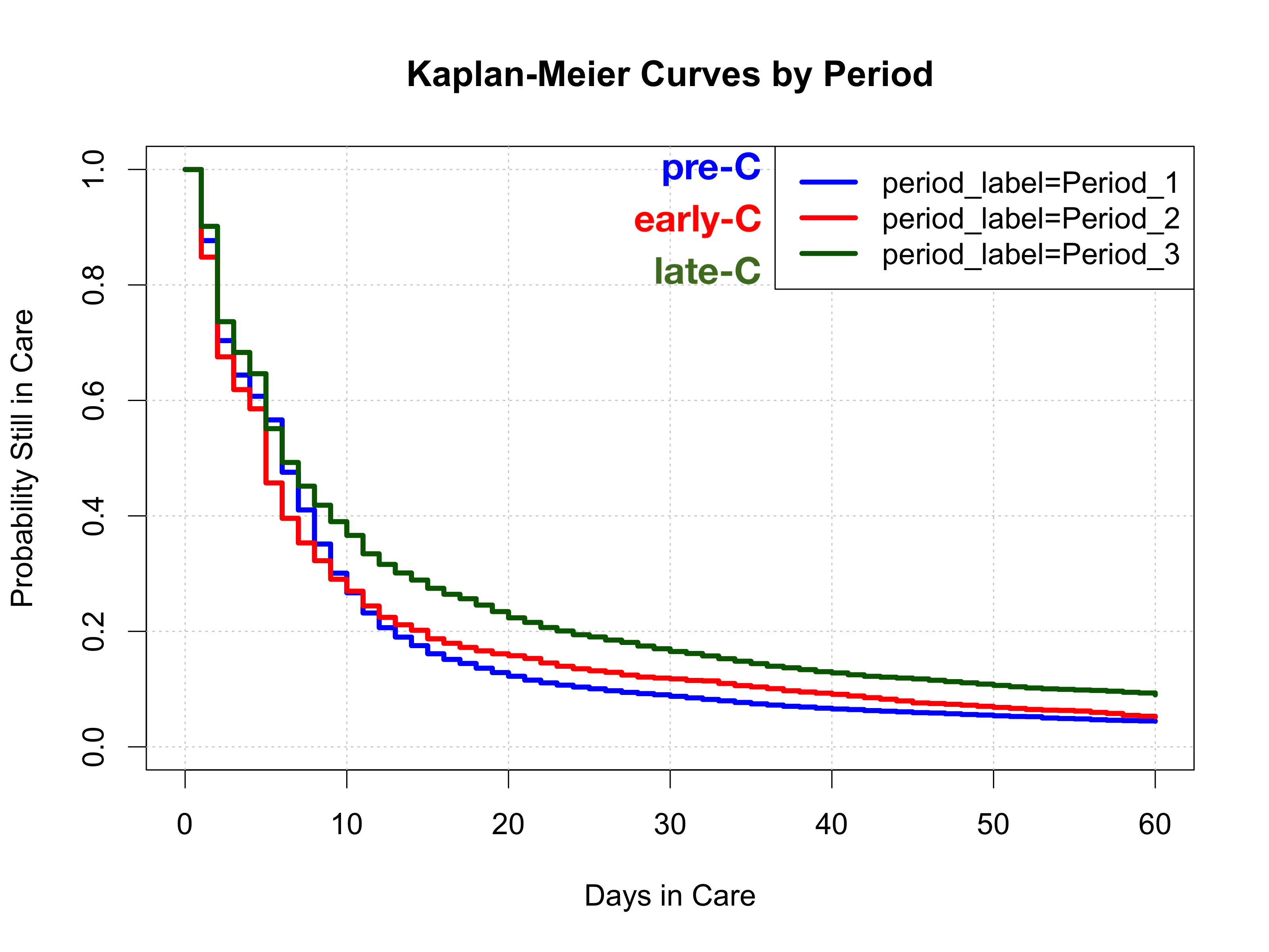
Fig 1. Kaplan-Meier curves by period.

We first consider the Kaplan-Meier curves, showing the fraction of animals continuing in care (Fig 1). These are more informative than mean LOS changes. They allow inspection of the early, intermediate, and long ranges of days in care. Compared to pre-C, early-C sees fewer dogs continuing in care in the first few days. Around day 10, early-C crosses over to more dogs in care than pre-C and this persists for longer stays. Late-C sees more dogs continuing in care from the very beginning, and the gap from previous periods grows in the range of 10-30 days in care.

Note that the median would be misleading in this case. It would show early-C as the shortest median LOS, with pre-C and late-C tied, hiding the insight we gain by examining the full Kaplan-Meier curve.

The full Kaplan-Meier curve also allows the computation of remaining LOS conditional on elapsed days in care⁴. This answers an important question for animals already in care: Knowing that an animal has been in care for x days, what is the expected remaining length of stay for this animal?

There are twice as many dogs experiencing long stays (e.g., at 40 or 60 days in Fig 1) in late-C than pre-C, which translates to more long residents in the in-care population. 

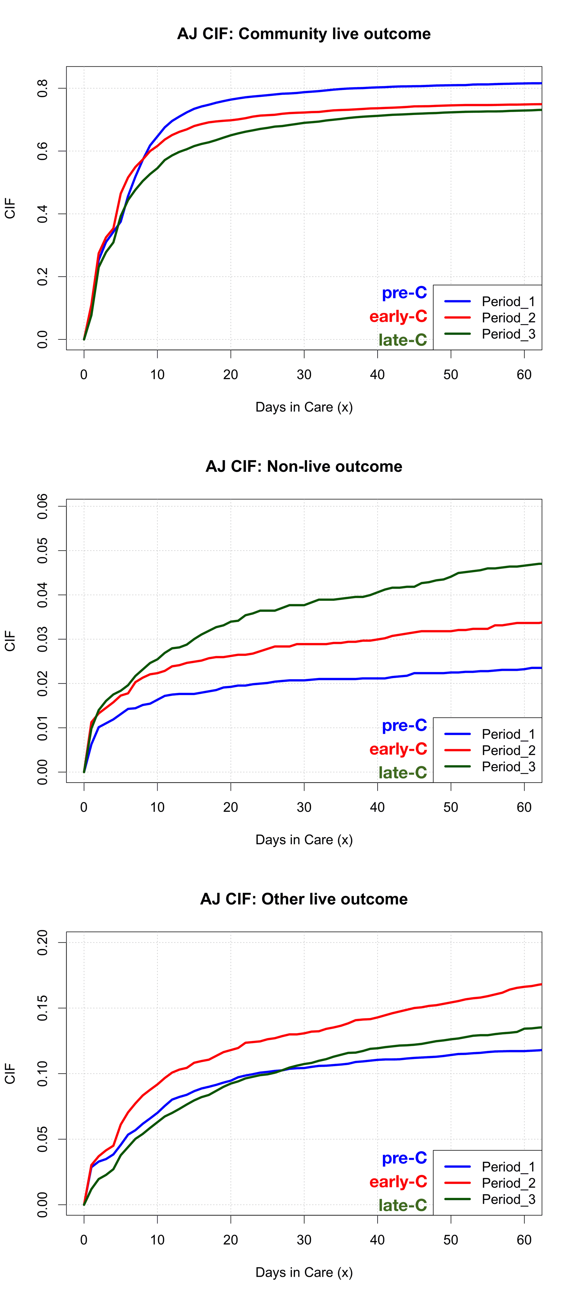
Fig 2. CIFs by period for each outcome type. Top: Community live outcome. Middle: Non-live outcome. Bottom: Transfer or other live outcome.

We examine CIFs by period, with one chart for each outcome type (Fig 2). For community live outcomes, early-C has faster outcomes than pre-C in the first few days, but early-C crosses over to slower outcomes (cumulatively) at day 8 and the gap from pre-C continues to grow until about day 20. The gap stabilizes thereafter, with early-C achieving a lower final incidence of community live outcomes than pre-C. In late-C there is no early period of faster outcomes, and the slowdown in outcomes is even more pronounced between 8 and 20 days in care. The ultimate incidence declines further.

For non-live outcomes, early-C shows higher cumulative incidence than pre-C, with the difference occurring primarily in the first 2-3 weeks. Thereafter, early-C and pre-C grow slowly in parallel. Late-C shows higher cumulative incidence than early-C from day 3 on, and the gap grows rapidly in the first 3 weeks and slowly thereafter. The ultimate incidence of non-live outcomes remains low by national standards – but long residents accumulate, as the Kaplan-Meier curves showed in Fig 1.

Other live outcomes consist predominantly of transfers. Early-C shows higher cumulative incidence from day two on, and the gap grows. Late-C initially shows slower incidence than the previous two periods, i.e., in the early stay days there are fewer transfers. By day 27, there is a pickup in transfers, cumulative exceeding pre-C but remaining well below early-C.

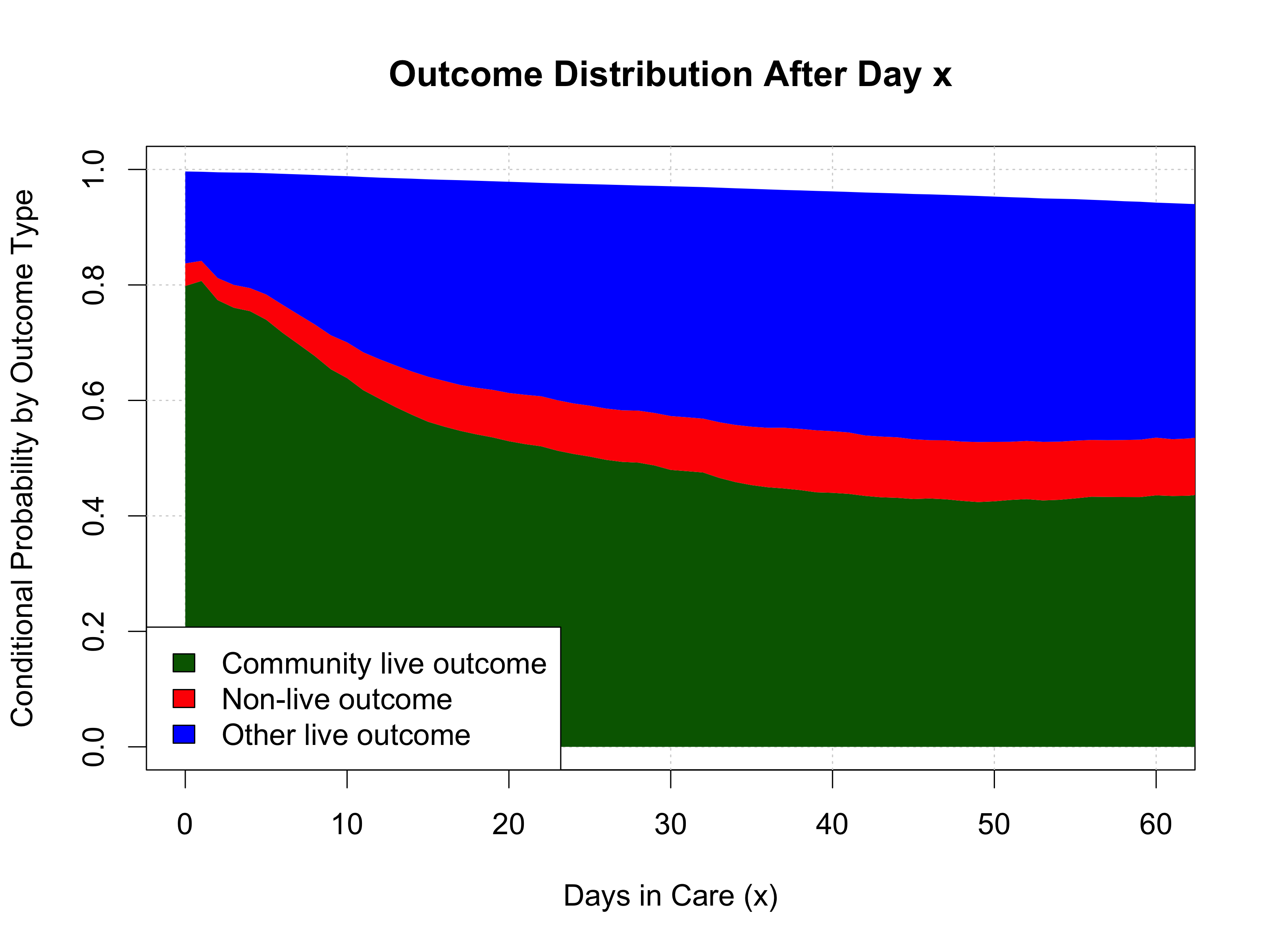
Fig 3. Outcome type conditional on elapsed days in care (all periods aggregated)

The CIFs allow the computation of ultimate outcome type probability for animals already in care, conditional on elapsed days in care. We first consider these aggregated over the three periods (Fig 3). The values at 0 days are the outcome probabilities at intake. Conditional on elapsed days in care up to about 25, the probability of an ultimate community live outcome decreases; nonlive outcome increases; and transfer also increases. This trend is expected, because of a sorting effect, with kennel stress or public perception of dogs with longer stays also possible factors.  However, from that point on, the probabilities remain stable. A dog with 60 days in care has similar probabilities of each outcome type as a dog with 25 days in care. It is possible that multiple offsetting factors are at work (e.g., kennel stress offset by more intensive marketing) and that period effects offset each other.

The chart has a non-rectangular form, with a thin wedge missing at the top. This wedge represents the dogs continuing in care at 1 year, an upper bound set in the settings file. A bound is useful to avoid outliers and compute restricted means from Kaplan-Meier fits. We may, in the future, treat this as an outcome type of its own.

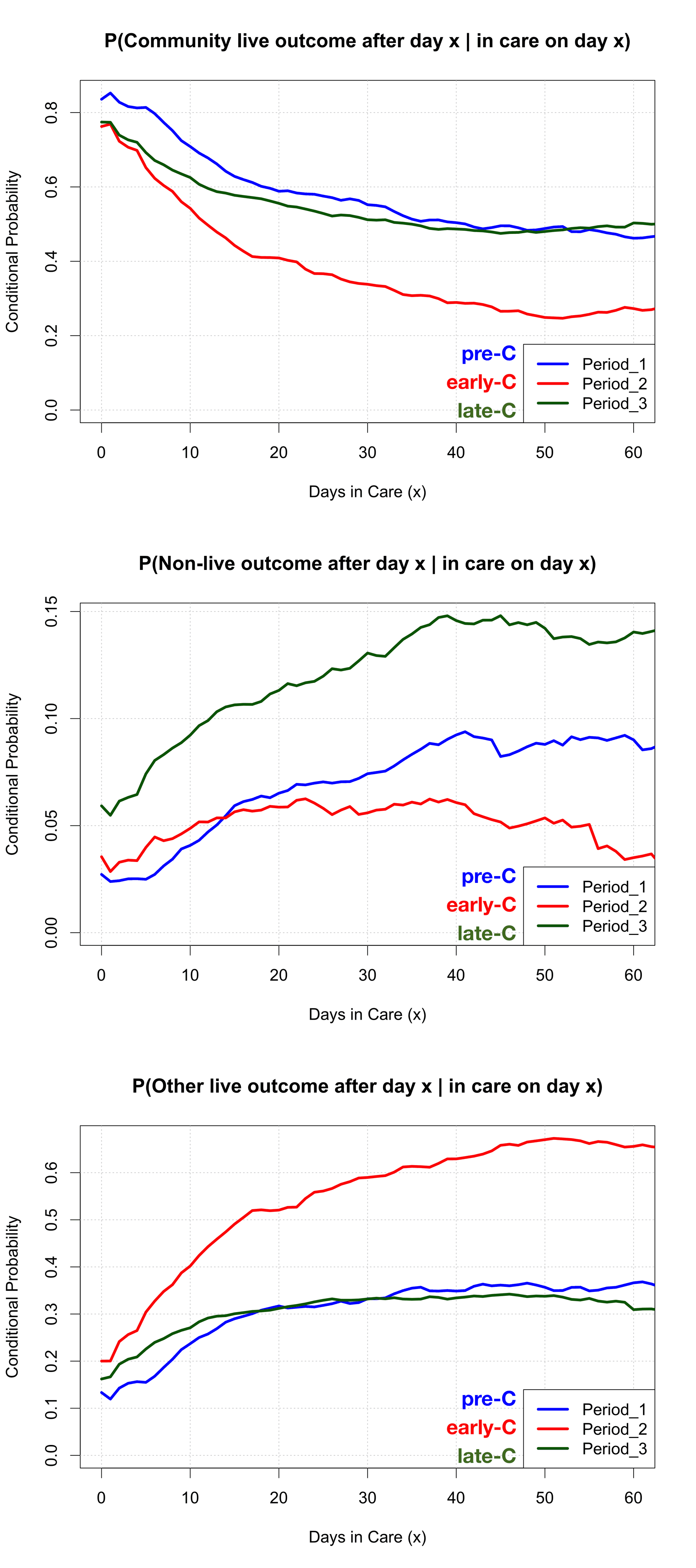
Fig 4. Outcome conditional on days in care, by period. Top: Community live outcome. Middle: Non-live outcome. Bottom: Transfer or other live outcome.

Examining conditional probabilities of each outcome type by period (Fig 4), we see that the stability in the right portion of Fig 3 is in part the result of periods offsetting each other, and it does not hold for each period separately.

There is a lower probability of community live outcome at intake during early-C relative to pre-C. As days in care increase, the probabilities decline and the gap grows. At 50 days of stay, a dog is half as like to be adopted during early-C as during pre-C. Late-C matches early-C at intake but drifts to higher conditional probabilities for longer stays. However, late-C also has higher probabilities of non-live outcome than the other two periods at intake, and that probability grows with days in care for the first 5 weeks of stay.

For transfers or other live outcomes, early-C has the highest transfer probability at intake, and that probability exceeds 1/2 at day 16 and 2/3 at day 50. In early-C, then, once a dog becomes a long resident it is very likely to go to rescue. But in late-C the transfer probability at intake eases back to a value between those of pre-C and early-C, and by 20 days in care late-C looks more like pre-C, i.e., has more limited transfer prospects.

Discussion and Conclusions

OC was a very accomplished shelter pre-COVID, having moved to modern facilities in early 2018. In early-C, the configuration of county policies resulted in slow adoptions for longer resident dogs and an increased reliance on transfers. This was manageable in the favorable early-C environment: There were substantially lower intakes, high demand for adoptions (which got the fast and intermediate track dogs out quickly), and high capacity in rescue organizations, including fosters who were working from home. As a result, the census count remained within capacity, and the live release rate dropped only slightly.

But in late-C the environment was less favorable. Though intakes remained below pre-C levels, they rose relative to early-C. Rescues were saturated and had less capacity once some workers returned to their workplaces. In this environment, the COVID-era policies led to further accumulation of long residents and dramatically higher census counts. By October 2023 (i.e., a period subsequent to the late-C period studied here), some dogs were housed in temporary trailers in a back parking lot. Dogs with longer stays were facing worse outcomes.

A nearby fire on November 7, 2023, motivated national organizations to transfer approximately 100 dogs out of the shelter and community members to assist with adoptions and fostering. From 313 dogs in care on November 6; only 153 remained on November 30. This alleviated overcrowding and allowed programmatic improvements. In 2024-2025, the gradual restoration of visitor access, staffing levels, and volunteering averted the reoccurrence of the 2022-2023 impasse.

While dog demographics changed through the COVID pandemic period, changes in LOS through the COVID period are observed even after accounting for dog size and age either as covariates⁴ or via stratification³.

In conclusion, shelters can benefit from examining LOS variation over calendar periods and across shelters. But historical shelter computations of LOS for a given period based only on animals with outcomes in that period are misleading and, notably, fail to detect the accumulation of long-stay animals continuing in care. Instead, Kaplan-Meier fits with left-truncation and right-censoring produce detailed view of LOS that shows localized shifts. From the Kaplan-Meier curves, the remaining LOS for animals already in care can be computed ⁴. Left-truncation and right-censoring can also be applied in Aalen-Johansen fits to produce the cumulative incidence function for each outcome type. These can then be used to derive the probability of each outcome type for animals already in care.

References

1. The Association of Shelter Veterinarians. The Guidelines for Standards of Care in Animal Shelters: Second Edition. Journal of Shelter Medicine and Community Animal Health. 2022;1(S1):S1. doi:10.56771/ASVguidelines.2022
2. Reduce Length of Stay. Koret Shelter Medicine Program. May 21, 2025. Accessed September 23, 2025. https://www.sheltermedicine.com/library/resources/length-of-stay-los
3. Mavrovouniotis ML. Use of Kaplan-Meier and Cox regressions in the distribution of length of stay in animal shelters for pre-specified calendar periods: Definition, computation, and examples of dog length of stay in Orange County California. PLOS ONE. 2026;21(1):e0342102. doi:10.1371/journal.pone.0342102
4. Mavrovouniotis ML. Distribution of Length of Stay and Its Variation by Calendar Period in Animal Shelters. In: Veterinary Information Network; 2026:456-459. https://www.researchgate.net/publication/403852994_Distribution_of_Length_of_Stay_and_Its_Variation_by_Calendar_Period_in_Animal_Shelters
5. Grand Jury OC. Grand Jury Report on Orange County Animal Care issued in 2023. Published online October 7, 2025. doi:10.5281/zenodo.17288953
6. Orange County Animal Care (California) shelter Intakes & Outcomes 20180101-20241020. Published online February 4, 2025. doi:10.6084/m9.figshare.28347134.v1
7. Therneau TM, until 2009) TL (original S >R port and R maintainer, Elizabeth A, Cynthia C. survival: Survival Analysis. Published online December 17, 2024. Accessed May 19, 2025. https://cran.r-project.org/web/packages/survival/index.html
8. Aalen OO, Johansen S. An Empirical Transition Matrix for Non-Homogeneous Markov Chains Based on Censored Observations. Scandinavian Journal of Statistics. 1978;5(3):141-150.
Published
Issue
Section
License
Copyright (c) 2026 Michael Mavrovouniotis
This work is licensed under a Creative Commons Attribution 4.0 International License.